Nerd Sniping - the Infinite Grid of Resistors

In this file we formalize the answer and related results to xkcd's "nerd sniping" question

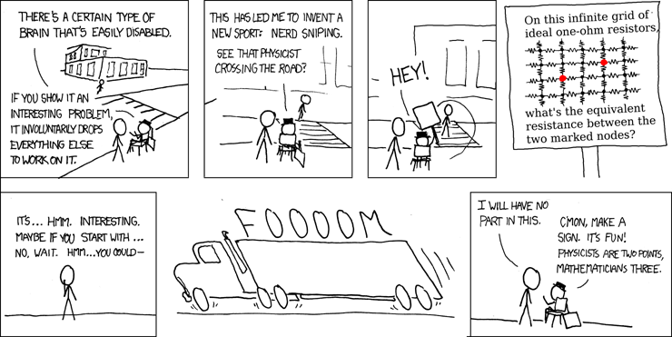
Here we state the problem in a more general form in aribtrary dimensions: On the $n$-dimensional grid where each neighboring nodes are connected by an one-ohm resistor, what is the equivalent resistance between the two marked nodes?

This file formalizes the following result

• The translation to a formal mathematical problem and proof of the unique solution (if exists).
• The general formula in arbitrary dimensions and for any pair of specific nodes.
• Computation for the solution in the two-dimension case, and the answer to the original question.

Hopefully this can protect me from a car accident.

1. Mathematical Model

The equivalent resistance is computed by $V / I$, where $V$ is the electrical potential difference between the two nodes, and $I$ is the current into one node and equally out from the other. Throughout the file, we will assume the standard units (ohm, volt, and amp) and omit them from formulas. By this convention, if we fix the input current to 1, the equivalent resistance is equal to the potential difference.

Once voltage is applied to the two nodes, there are two laws that determine the current and the potential:

• Ohm's law: $R = V / I$ for any segment of the curcuit. Since every segment between two neighboring nodes has a resistance of 1, we can simplify this to $I(p, q) = U(p) - U(q)$ for any pair of neighboring nodes $p$ and $q$, where $U(p)$ is the potential at node $p$, and $I(p, q)$ is the current from $p$ to $q$.
• Kirchhoff's current law: the signed sum of currents at a node is zero. In our $n$-dimensional grid, each node has $2n$ currents with neighbors, and possibly one external current input. In our convention, the current out from the node is positive, and the current into the node is negative.

We can combine the two laws to form a formula about potentials $U(p)$ and external currents $I(p)$, whih we simply call "Kirchhoff's law" in the code: $$ \left(\sum_{i=0}^{n-1} U(p + e_i) - U(p)\right) + \left(\sum_{i=0}^{n-1} U(p - e_i) - U(p)\right) = I(p) $$ where $e_i$ are unit vectors in each direction.

In addition to the laws, we add another constraint: the potential as a function of node should be bounded. This is to rule out existence of a global external electrical field, where there is no external current input, but internal current is still induced.

We group these contraints in IsValidCircuit I U, where I : (Fin n → ℤ) → ℝ is the external current at each node, and U : (Fin n → ℤ) → ℝ is the potential at each node.

structure IsValidCircuit {n : ℕ} (cur pot : (Fin n → ℤ) → ℝ) : Prop

IsValidCircuit I U means the external current input I and potential U forms a valid circuit over the infinite grid.

• kirchhoff (x : Fin n → ℤ) : ∑ k : Fin n, (pot (x - Pi.single k 1) - pot x) + ∑ k : Fin n, (pot (x + Pi.single k 1) - pot x) = cur x

  A valid circuit should follow Ohm's law and Kirchhoff's law.

• bddBelow : BddBelow (Set.range pot)

  A valid potential function should be bounded below.

• bddAbove : BddAbove (Set.range pot)

  A valid potential function should be bounded above.

Once we have the definition of a valid circuit, the formalization of equivalent resistance is to ask the potential difference given a pair of unit input current. We use unitCur c to express a current input function that consists of a unit input at node c : Fin n → ℤ. The formalized question them becomes: given a valid circuit for (unitCur 0 - unitCur x), find the potential between 0 and x.

def unitCur {n : ℕ} (c x : Fin n → ℤ) : ℝ

The unit input current at node c, as a function over nodes.

Equations

• unitCur c x = Pi.single c 1 x

noncomputable def equivResistance {n : ℕ} (x : Fin n → ℤ) : Option ℝ

The definition of the solution. This definition uses Exists.choose to nonstructively return the return the potential difference for input current (unitCur 0 - unitCur x), and returns none. if no valid circuit exists. We will later show the existence of the valid circuit constructively, as well as their uniqueness.

Equations

• equivResistance x = if h : ∃ (pot : (Fin n → ℤ) → ℝ), IsValidCircuit (unitCur 0 - unitCur x) pot then some (h.choose x - h.choose 0) else none

2. Uniqueness of Solution

This section justifies the mathematical model by showing that its solution space is sub-singleton. This follows from the discrete version of Liouville's theorem applied to bounded harmonic function, which we will prove first.

Liouville's theorem says that if bounded function (above and below) satisfies the Laplace's equation everywhere (which is equivalent to Kirchhoff's law with null external current), then it is a constant function. There are stronger versions of this theorem (e.g. only requiring one-side boundedness, and only requiring a large portion of nodes to satisfy the equation), but the elementary version will suffice here.

We follow the proof posted at https://math.stackexchange.com/a/4452978/1197328

theorem liouville_lemma1 {n : ℕ} (f : (Fin n → ℤ) → ℝ) (hharmonic : ∀ (x : Fin n → ℤ), ∑ k : Fin n, (f (x - Pi.single k 1) - f x) + ∑ k : Fin n, (f (x + Pi.single k 1) - f x) = 0) (l : ℝ) (e : Fin n) (hbound : ∀ (x : Fin n → ℤ) (k : ℕ), ∑ i ∈ Finset.range k, f (x + i • Pi.single e 1) ≤ l) (x : Fin n → ℤ) : f x ≤ 0

Lemma 1 for Liouville's theorem: if a discrete harmonic function $f : \mathbb{Z}^n \to \mathbb{R}$ satisfies that for certain $L$ and a unit direction $e$ $$|f(x) + f(x + e) + f(x + 2e) + \cdots + f(x + ke)| \le L$$ for all $x$ and $k$, then $f$ is constantly 0. In the first version we shows the nonpositivity of $f$, and then use antisymmetry in the next version.

theorem liouville_lemma1' {n : ℕ} (f : (Fin n → ℤ) → ℝ) (hharmonic : ∀ (x : Fin n → ℤ), ∑ k : Fin n, (f (x - Pi.single k 1) - f x) + ∑ k : Fin n, (f (x + Pi.single k 1) - f x) = 0) (l : ℝ) (e : Fin n) (hbound : ∀ (x : Fin n → ℤ) (k : ℕ), |∑ i ∈ Finset.range k, f (x + i • Pi.single e 1)| ≤ l) : f = 0

Full lemma 1 for Liouville's theorem: use antisymmetry on the previous lemma.

theorem liouville_neighbor {n : ℕ} (f : (Fin n → ℤ) → ℝ) (hharmonic : ∀ (x : Fin n → ℤ), ∑ k : Fin n, (f (x - Pi.single k 1) - f x) + ∑ k : Fin n, (f (x + Pi.single k 1) - f x) = 0) (hbelow : BddBelow (Set.range f)) (habove : BddAbove (Set.range f)) (e : Fin n) (x : Fin n → ℤ) : f x = f (x + Pi.single e 1)

Liouville's theorem for two neighboring points: for a harmonic $f$, set $g(x) = f(x + e) - f(x)$, then $g$ satisfies the condition for lemma 1, and thus constantly zero, showing $f(x + e) = f(x)$.

theorem liouville_line {n : ℕ} (f : (Fin n → ℤ) → ℝ) (hharmonic : ∀ (x : Fin n → ℤ), ∑ k : Fin n, (f (x - Pi.single k 1) - f x) + ∑ k : Fin n, (f (x + Pi.single k 1) - f x) = 0) (hbelow : BddBelow (Set.range f)) (habove : BddAbove (Set.range f)) (e : Fin n) (l : ℤ) (x : Fin n → ℤ) : f x = f (x + Pi.single e l)

By inductiog on the previous lemma, a bounded harmonic function is constant on a line in any direction.

theorem liouville {n : ℕ} (f : (Fin n → ℤ) → ℝ) (hharmonic : ∀ (x : Fin n → ℤ), ∑ k : Fin n, (f (x - Pi.single k 1) - f x) + ∑ k : Fin n, (f (x + Pi.single k 1) - f x) = 0) (hbelow : BddBelow (Set.range f)) (habove : BddAbove (Set.range f)) (x y : Fin n → ℤ) : f x = f y

By induction on the previous lemma, we get Liouville's theorem: a bounded harmonic function is constant globally.

theorem isValidCircuit_zero {n : ℕ} [NeZero n] {pot : (Fin n → ℤ) → ℝ} : IsValidCircuit 0 pot ↔ ∃ (c : ℝ), pot = fun (x : Fin n → ℤ) => c

Equivalent to Liouville's theorem, the only valid potential functions for null external current are constant functions.

theorem isValidCircuit_unique {n : ℕ} [NeZero n] {cur a b : (Fin n → ℤ) → ℝ} (ha : IsValidCircuit cur a) (hb : IsValidCircuit cur b) : ∃ (c : ℝ), a - b = fun (x : Fin n → ℤ) => c

For any specific external current functions, the valid potential function, if exists, is unique up to a constant.

theorem equivResistance_eq {n : ℕ} [NeZero n] {x : Fin n → ℤ} {pot : (Fin n → ℤ) → ℝ} (h : IsValidCircuit (unitCur 0 - unitCur x) pot) : equivResistance x = some (pot x - pot 0)

Since the uniqueness of the potential function, the infinite grid question can be answered whenever a valid potential function is found.

3. Fourier Transform: a Potential Solution

In this section, we construct a function φ that represents the potential function corresponding to a singleton external current (as opposite to a pair of in/out current as we have been discussing). Physically, such current dissipates via the grid to infinity. It is almost a valid solution to IsValidCircuit (unitCur 0) φ, but it is not necessarily bounded. We will further discuss its asymptotic behavior in the next section.

The construction of φ is obtained by taking an inverse Fourier transform of a certain function. The full derivation via Fourier transform is omitted, but you can get the general idea by the proof here.

theorem fourier_unitCur {n : ℕ} (x : Fin n → ℤ) : unitCur 0 x = (2 * Real.pi)⁻¹ ^ n * ∫ (w : Fin n → ℝ) in Set.Icc (fun (x : Fin n) => -Real.pi) fun (x : Fin n) => Real.pi, Real.cos (∑ i : Fin n, ↑(x i) * w i)

We compute the discrete Fourier transform of unitCur 0, then state the result using inverse Fourier transform to recover unitCur 0, which is a integral over a hypercube $$ \varphi (x_0, x_1,\cdots,x_{n-1}) = \frac{1}{(2\pi)^n} \int_{[-\pi, \pi]^n} \left(\cos \sum_i x_i w_i\right) dw $$

noncomputable def φ {n : ℕ} (x : Fin n → ℤ) : ℝ

Then we define function φ also as a similar inverse Fourier transform $$ \varphi (x_0, x_1,\cdots,x_{n-1}) = \frac{1}{(2\pi)^n} \int_{[-\pi, \pi]^n} \frac{1 - \cos \sum_i x_i w_i}{\sum_i 2 - 2\cos w_i} dw $$

Equations

• One or more equations did not get rendered due to their size.

We start exploring some basic properties of φ:

• φ 0 = 0.
• φ is non-negative, and therefore bounded below.
• φ has mirror symmetry along any axies. (φ_reflect)
• φ is symmetric for coordinate permutation. (φ_perm)

@[simp]

theorem φ_zero {n : ℕ} : φ 0 = 0

theorem φ_nonneg {n : ℕ} (x : Fin n → ℤ) : 0 ≤ φ x

theorem bddBelow_φ {n : ℕ} : BddBelow (Set.range φ)

@[simp]

theorem φ_reflect {n : ℕ} (x : Fin n → ℤ) (i : Fin n) : φ (Function.update x i (-x i)) = φ x

@[simp]

theorem φ_neg_0 (x y : ℤ) : φ ![-x, y] = φ ![x, y]

@[simp]

theorem φ_neg_1 (x y : ℤ) : φ ![x, -y] = φ ![x, y]

@[simp]

theorem φ_neg {n : ℕ} (x : Fin n → ℤ) : φ (-x) = φ x

@[simp]

theorem φ_perm {n : ℕ} (x : Fin n → ℤ) (p : Fin n ≃ Fin n) : φ (x ∘ ⇑p) = φ x

theorem φ_single_perm {n : ℕ} (e e' : Fin n) (l : ℤ) : φ (Pi.single e l) = φ (Pi.single e' l)

theorem φ_swap (x y : ℤ) : φ ![x, y] = φ ![y, x]

Special case for swapping coordinates in the 2D case.

We should justify that the integral in φ actually makes sense. This is not trivial: the integrant has an unremovable singularity at 0. It turns out that this singularity is bounded, so you can either treat it as 0 using Lean's junk value, or remove the singularity from integration.

theorem integrable_φ {n : ℕ} [NeZero n] (x : Fin n → ℤ) : MeasureTheory.IntegrableOn (fun (w : Fin n → ℝ) => (1 - Real.cos (∑ k : Fin n, ↑(x k) * w k)) / ∑ k : Fin n, (2 - 2 * Real.cos (w k))) (Set.Icc (fun (x : Fin n) => -Real.pi) fun (x : Fin n) => Real.pi) MeasureTheory.volume

Lastly, we show that φ satisfies Kirchhoff's law for singleton unit current, making it an almost solution. As a corollary, we compute the value of φ eᵢ for a unit vector eᵢ in φ_off_center using Kirchhoff's law and symmetry.

theorem φ_kirchhoff {n : ℕ} [NeZero n] (x : Fin n → ℤ) : ∑ k : Fin n, (φ (x - Pi.single k 1) - φ x) + ∑ k : Fin n, (φ (x + Pi.single k 1) - φ x) = unitCur 0 x

theorem φ_2d_kirchhoff_of_ne_zero (x y : ℤ) (hxy : x ≠ 0 ∨ y ≠ 0) : 4 * φ ![x, y] = φ ![x - 1, y] + φ ![x + 1, y] + φ ![x, y - 1] + φ ![x, y + 1]

A specialized version of φ_kirchhoff for 2D and not at the center.

theorem φ_off_center {n : ℕ} (e : Fin n) : φ (Pi.single e 1) = (2 * ↑n)⁻¹

theorem φ_2d_1_0 : φ ![1, 0] = 4⁻¹

A specialized version of φ_off_center for 2D.

4. Asymptotic Behavior of φ

In this section, we show the asymptotic behavior of φ in different dimensions $n$:

• When $n \ge 3$, φ x is bounded
• When $n = 2$, φ x grows like $\log \lVert x \rVert$
• When $n = 1$, φ x grows linearly

Compare this to physical intuition: in a $n$-dimensional space, current density sourced from a point should decrease like ${\lVert x \rVert}^{-(n - 1)}$ (inverse-square law in 3D), and the potential, being the integral of t, should grow like ${\lVert x \rVert}^{-(n - 2)}$ except for $n = 2$, where the integral becomes $\log \lVert x \rVert$.

We start with the $n \ge 3$ case

theorem abs_φ_le {n : ℕ} (hn : 3 ≤ n) (x : Fin n → ℤ) : |φ x| ≤ (2 * Real.pi)⁻¹ ^ n * ∫ (w : Fin n → ℝ) in Set.Icc (fun (x : Fin n) => -Real.pi) fun (x : Fin n) => Real.pi, 1 / ∑ i : Fin n, (1 - Real.cos (w i))

For $n \ge 3$, it is possible to bound the integral by bounding the numerator to 1. This creates poles at 0, but it is still integrable.

theorem bddAbove_φ {n : ℕ} (hn : 3 ≤ n) : BddAbove (Set.range φ)

Thus φ is bounded above for $n \ge 3$.

We show the asymptotic behavior for $n = 2$ next. The precise statement we want to prove is: the function $g(x)$ defined below is bounded above and below

$$ g(x, y) = \varphi(x, y) - \frac{1}{4 \pi} \log (x^2 + y^2) = \varphi(x, y) - \frac{1}{2 \pi} \log \lVert (x, y) \rVert_2 $$

(This assumes the junk value $\log 0 = 0$, but a single point isn't important for the global bound)

We show this using a chain of asymptotic equivalences: $$ \varphi(x, y) \sim \iint_{[-\pi,\pi]^2} \frac{1-\cos (x u + y v)}{4 - (2 \cos u + 2 \cos v)}du dv $$ $$ \sim \iint_{u^2+v^2\le 1} \frac{1-\cos (x u + y v)}{4 - (2 \cos u + 2 \cos v)}du dv $$ $$ \sim \iint_{u^2+v^2\le 1} \frac{1-\cos (x u + y v)}{u^2 + v^2}du dv $$ $$ \sim \int_{r=0}^{\lVert (x, y) \rVert_2} \int_{\theta=-\pi}^{\pi} \frac{1-\cos (r \cos(\theta))}{r}dr d\theta $$ $$ \sim \log \lVert (x, y) \rVert_2 $$ where each equivalence means bounded difference between two sides after multiplying by some constants. The main idea here is that the logarithmic growth comes from the integration around the singularity, so we can carve out a small disk (a unit disk will suffice), and change to polar coordinates. The last equivalence is a property of Bessel function, which is proved at asymptotic_bessel.

theorem φ_2d (x : Fin 2 → ℤ) : φ x = (4 * Real.pi ^ 2)⁻¹ * ∫ (w : ℝ × ℝ) in Set.Icc (-Real.pi) Real.pi ×ˢ Set.Icc (-Real.pi) Real.pi, (1 - Real.cos (↑(x 0) * w.1 + ↑(x 1) * w.2)) / (4 - (2 * Real.cos w.1 + 2 * Real.cos w.2))

Specialize the integral to 2D case.

theorem eq_zero_of_φ_2d_deno_le_zero {p : ℝ × ℝ} (hp : p ∈ Set.Icc (-Real.pi) Real.pi ×ˢ Set.Icc (-Real.pi) Real.pi) (h : 4 - (2 * Real.cos p.1 + 2 * Real.cos p.2) ≤ 0) : p = 0

A common lemma we will use to determine that the only singularity is at 0.

theorem φ_integrable_2d (x : Fin 2 → ℤ) : MeasureTheory.IntegrableOn (fun (w : ℝ × ℝ) => (1 - Real.cos (↑(x 0) * w.1 + ↑(x 1) * w.2)) / (4 - (2 * Real.cos w.1 + 2 * Real.cos w.2))) (Set.Icc (-Real.pi) Real.pi ×ˢ Set.Icc (-Real.pi) Real.pi) MeasureTheory.volume

Specialize integrability to 2D.

theorem φ_integrable_2d' (x : Fin 2 → ℤ) : MeasureTheory.IntegrableOn (fun (w : ℝ × ℝ) => (1 - Real.cos (↑(x 0) * w.1 + ↑(x 1) * w.2)) / (w.1 ^ 2 + w.2 ^ 2)) (Set.Icc (-Real.pi) Real.pi ×ˢ Set.Icc (-Real.pi) Real.pi) MeasureTheory.volume

Integrability of an equivalent function we will use.

theorem integrable_bessel (x1 x2 : ℝ) : MeasureTheory.IntegrableOn (fun (p : ℝ × ℝ) => (1 - Real.cos (x1 * p.1 * Real.cos (p.2 - x2))) / p.1) (Set.Ioc 0 1 ×ˢ Set.Ioo (-Real.pi) Real.pi) (MeasureTheory.volume.prod MeasureTheory.volume)

Integrability related to Bessel function.

theorem disk_subset : {p : ℝ × ℝ | p.1 ^ 2 + p.2 ^ 2 ≤ 1} ⊆ Set.Icc (-1) 1 ×ˢ Set.Icc (-1) 1

The unit disk is a subset of the containing square.

theorem disk_subset' : {p : ℝ × ℝ | p.1 ^ 2 + p.2 ^ 2 ≤ 1} ⊆ Set.Icc (-Real.pi) Real.pi ×ˢ Set.Icc (-Real.pi) Real.pi

The unit disk is a subset of the original square to integrate on.

theorem φ_integral_change_deno : (fun (x : Fin 2 → ℤ) => (∫ (w : ℝ × ℝ) in {p : ℝ × ℝ | p.1 ^ 2 + p.2 ^ 2 ≤ 1}, (1 - Real.cos (↑(x 0) * w.1 + ↑(x 1) * w.2)) / (4 - (2 * Real.cos w.1 + 2 * Real.cos w.2))) - ∫ (w : ℝ × ℝ) in {p : ℝ × ℝ | p.1 ^ 2 + p.2 ^ 2 ≤ 1}, (1 - Real.cos (↑(x 0) * w.1 + ↑(x 1) * w.2)) / (w.1 ^ 2 + w.2 ^ 2)) =O[Filter.cofinite] 1

Equivalence when we change the denominator of the integrant.

theorem φ_equiv_log_2d : (fun (x : Fin 2 → ℤ) => φ x - (4 * Real.pi)⁻¹ * Real.log (↑(x 0) ^ 2 + ↑(x 1) ^ 2)) =O[Filter.cofinite] 1

Logarithmatic equivalence for φ in 2D.

theorem φ_2d_sub_log_bounded : ∃ (c : ℝ), ∀ (x : Fin 2 → ℤ), |φ x - (4 * Real.pi)⁻¹ * Real.log (↑(x 0) ^ 2 + ↑(x 1) ^ 2)| ≤ c

Restating logarithmatic equivalence for φ in 2D in terms of a global bound.

Finally, we turn to the 1D case. We can direclty compute using induction that $$ \varphi (x) = \frac{1}{2} |x| $$ and thus φ grows linearly in 1D case.

theorem φ_1d_nat (x : ℕ) : φ ![↑x] = 2⁻¹ * ↑x

theorem φ_1d (x : ℤ) : φ ![x] = 2⁻¹ * ↑|x|

theorem φ_1d' (x : Fin 1 → ℤ) : φ x = 2⁻¹ * ↑|x 0|

5. Solution to IsValidCircuit

In this section, we prove IsValidCircuit (unitCur a - unitCur b) (fun x ↦ φ (x - a) - φ (x - b)). The two conditions for this are now within reach:

• Because of linarity, Kirchhoff's law holds for any linear combination of φ.
• The difference between two φ is bounded thanks to the tame asymptotics.

The hardest part in this is to show the boundedness for 2D cases. We will first show that the difference between two log-like functions are bounded, then transfer the result to φ.

theorem log_shift_equiv (a b : ℤ) : (fun (x : Fin 2 → ℤ) => Real.log ((↑(x 0) + ↑a) ^ 2 + (↑(x 1) + ↑b) ^ 2) - Real.log (↑(x 0) ^ 2 + ↑(x 1) ^ 2)) =O[Filter.cofinite] 1

The difference between $log \lVert x \rVert_2^2$ and $log \lVert x+(a,b) \rVert_2^2$ is bounded.

theorem log_shift_equiv' (a b c d : ℤ) : (fun (x : Fin 2 → ℤ) => Real.log ((↑(x 0) - ↑a) ^ 2 + (↑(x 1) - ↑b) ^ 2) - Real.log ((↑(x 0) - ↑c) ^ 2 + (↑(x 1) - ↑d) ^ 2)) =O[Filter.cofinite] 1

Generalize the previous statement to any pair of points.

theorem bound_φ_2d (a b : Fin 2 → ℤ) : ∃ (c : ℝ), ∀ (x : Fin 2 → ℤ), |φ (x - a) - φ (x - b)| ≤ c

The difference between two φ in 2D is bounded.

theorem bound_φ_1d (a b : Fin 1 → ℤ) : ∃ (c : ℝ), ∀ (x : Fin 1 → ℤ), |φ (x - a) - φ (x - b)| ≤ c

We also show the difference between two φ in 1D as a direct result of linear growth.

theorem isValidCircuit_φ {n : ℕ} [NeZero n] (a b : Fin n → ℤ) : IsValidCircuit (unitCur a - unitCur b) fun (x : Fin n → ℤ) => φ (x - a) - φ (x - b)

Combining all cases above, we show that fun x ↦ φ (x - a) - φ (x - b) is the unique solution to IsValidCircuit (unitCur a - unitCur b).

theorem equivResistance_eq_two_mul_φ {n : ℕ} [NeZero n] (x : Fin n → ℤ) : equivResistance x = some (2 * φ x)

And as an immediate corollary, the equivalent resistance is two times φ in all cases.

theorem equivResistance_off_center {n : ℕ} [NeZero n] (e : Fin n) : equivResistance (Pi.single e 1) = some (↑n)⁻¹

Applying this to the neighbor of the center, we get that the equivalent resistance between two neighboring points is $1 / n$.

6. Calculation for the 2D case

In this section, we derive more closed-form results for the 2D case, and answers the original nerd sniping question.

The key result is that φ ![x, x] along the diagonal line has a simple formula $$ \varphi(x, x) = \frac{1}{\pi}\left(1 + \frac{1}{3} + \frac{1}{5} + \cdots + \frac{1}{2x - 1}\right) $$

Combining with the known value φ ![1, 0] = 4⁻¹, it is possible to calculate any φ ![x, y] using symmetry and Kirchhoff's law, and they will be some rational combinations of $1$ and $π$.

To calculate the integral on the diagonal line, we expand the integral domain from the square to the diamond $(2\pi, 0) - (0, 2\pi) - (-2\pi, 0) - (0, -2π)$. Because of the periodicity of the integrand, this simply doubles the resulting value. We then change the variable to rotate it by 45 degrees. The new integral can have variables separated, allowing us to calculate it.

This process is unfortunately tedious to formalize. We start with defining the diamond region, as well as the four triangles triangleU, triangleD, triangleL, and triangleR between the diamand and the square.

def triangleU : Set (ℝ × ℝ)

Equations

• triangleU = {p : ℝ × ℝ | Real.pi ≤ p.2 ∧ p.1 + p.2 ≤ 2 * Real.pi ∧ p.2 - p.1 ≤ 2 * Real.pi}

def triangleD : Set (ℝ × ℝ)

Equations

• triangleD = {p : ℝ × ℝ | p.2 ≤ -Real.pi ∧ -2 * Real.pi ≤ p.1 + p.2 ∧ -2 * Real.pi ≤ p.2 - p.1}

def triangleL : Set (ℝ × ℝ)

Equations

• triangleL = {p : ℝ × ℝ | p.1 ≤ -Real.pi ∧ -2 * Real.pi ≤ p.1 + p.2 ∧ p.2 - p.1 ≤ 2 * Real.pi}

def triangleR : Set (ℝ × ℝ)

Equations

• triangleR = {p : ℝ × ℝ | Real.pi ≤ p.1 ∧ p.1 + p.2 ≤ 2 * Real.pi ∧ -2 * Real.pi ≤ p.2 - p.1}

def diamond : Set (ℝ × ℝ)

Equations

• diamond = {p : ℝ × ℝ | p.1 + p.2 ≤ 2 * Real.pi ∧ -2 * Real.pi ≤ p.1 + p.2 ∧ p.2 - p.1 ≤ 2 * Real.pi ∧ -2 * Real.pi ≤ p.2 - p.1}

theorem diamond_decomp : diamond = triangleU ∪ triangleD ∪ triangleL ∪ triangleR ∪ Set.Icc (-Real.pi) Real.pi ×ˢ Set.Icc (-Real.pi) Real.pi

diamand is the union of the square and the four triangles.

theorem square_comp : Set.Icc (-Real.pi) Real.pi ×ˢ Set.Icc (-Real.pi) Real.pi = ⇑(MeasurableEquiv.addRight (0, -2 * Real.pi)) '' triangleU ∪ ⇑(MeasurableEquiv.addRight (0, 2 * Real.pi)) '' triangleD ∪ ⇑(MeasurableEquiv.addRight (2 * Real.pi, 0)) '' triangleL ∪ ⇑(MeasurableEquiv.addRight (-2 * Real.pi, 0)) '' triangleR

The square is the union of the same four triangles after translation.

We show that the integration in φ makes sense in all these regions.

theorem φ_integrable_mapU (x : Fin 2 → ℤ) : MeasureTheory.IntegrableOn (fun (w : ℝ × ℝ) => (1 - Real.cos (↑(x 0) * w.1 + ↑(x 1) * w.2)) / (4 - (2 * Real.cos w.1 + 2 * Real.cos w.2))) (⇑(MeasurableEquiv.addRight (0, -2 * Real.pi)) '' triangleU) MeasureTheory.volume

theorem φ_integrable_mapD (x : Fin 2 → ℤ) : MeasureTheory.IntegrableOn (fun (w : ℝ × ℝ) => (1 - Real.cos (↑(x 0) * w.1 + ↑(x 1) * w.2)) / (4 - (2 * Real.cos w.1 + 2 * Real.cos w.2))) (⇑(MeasurableEquiv.addRight (0, 2 * Real.pi)) '' triangleD) MeasureTheory.volume

theorem φ_integrable_mapL (x : Fin 2 → ℤ) : MeasureTheory.IntegrableOn (fun (w : ℝ × ℝ) => (1 - Real.cos (↑(x 0) * w.1 + ↑(x 1) * w.2)) / (4 - (2 * Real.cos w.1 + 2 * Real.cos w.2))) (⇑(MeasurableEquiv.addRight (2 * Real.pi, 0)) '' triangleL) MeasureTheory.volume

theorem φ_integrable_mapR (x : Fin 2 → ℤ) : MeasureTheory.IntegrableOn (fun (w : ℝ × ℝ) => (1 - Real.cos (↑(x 0) * w.1 + ↑(x 1) * w.2)) / (4 - (2 * Real.cos w.1 + 2 * Real.cos w.2))) (⇑(MeasurableEquiv.addRight (-2 * Real.pi, 0)) '' triangleR) MeasureTheory.volume

theorem φ_integrable_U (x : Fin 2 → ℤ) : MeasureTheory.IntegrableOn (fun (w : ℝ × ℝ) => (1 - Real.cos (↑(x 0) * w.1 + ↑(x 1) * w.2)) / (4 - (2 * Real.cos w.1 + 2 * Real.cos w.2))) triangleU MeasureTheory.volume

theorem φ_integrable_D (x : Fin 2 → ℤ) : MeasureTheory.IntegrableOn (fun (w : ℝ × ℝ) => (1 - Real.cos (↑(x 0) * w.1 + ↑(x 1) * w.2)) / (4 - (2 * Real.cos w.1 + 2 * Real.cos w.2))) triangleD MeasureTheory.volume

theorem φ_integrable_L (x : Fin 2 → ℤ) : MeasureTheory.IntegrableOn (fun (w : ℝ × ℝ) => (1 - Real.cos (↑(x 0) * w.1 + ↑(x 1) * w.2)) / (4 - (2 * Real.cos w.1 + 2 * Real.cos w.2))) triangleL MeasureTheory.volume

theorem φ_integrable_R (x : Fin 2 → ℤ) : MeasureTheory.IntegrableOn (fun (w : ℝ × ℝ) => (1 - Real.cos (↑(x 0) * w.1 + ↑(x 1) * w.2)) / (4 - (2 * Real.cos w.1 + 2 * Real.cos w.2))) triangleR MeasureTheory.volume

theorem φ_integrable_diamond (x : Fin 2 → ℤ) : MeasureTheory.IntegrableOn (fun (w : ℝ × ℝ) => (1 - Real.cos (↑(x 0) * w.1 + ↑(x 1) * w.2)) / (4 - (2 * Real.cos w.1 + 2 * Real.cos w.2))) diamond MeasureTheory.volume

We then show there is no overlap between regions.

theorem disjoint_U_D : MeasureTheory.AEDisjoint MeasureTheory.volume triangleU triangleD

theorem disjoint_U_L : MeasureTheory.AEDisjoint MeasureTheory.volume triangleU triangleL

theorem disjoint_D_L : MeasureTheory.AEDisjoint MeasureTheory.volume triangleD triangleL

theorem disjoint_U_R : MeasureTheory.AEDisjoint MeasureTheory.volume triangleU triangleR

theorem disjoint_D_R : MeasureTheory.AEDisjoint MeasureTheory.volume triangleD triangleR

theorem disjoint_L_R : MeasureTheory.AEDisjoint MeasureTheory.volume triangleL triangleR

theorem disjoint_U_sq : MeasureTheory.AEDisjoint MeasureTheory.volume triangleU (Set.Icc (-Real.pi) Real.pi ×ˢ Set.Icc (-Real.pi) Real.pi)

theorem disjoint_D_sq : MeasureTheory.AEDisjoint MeasureTheory.volume triangleD (Set.Icc (-Real.pi) Real.pi ×ˢ Set.Icc (-Real.pi) Real.pi)

theorem disjoint_L_sq : MeasureTheory.AEDisjoint MeasureTheory.volume triangleL (Set.Icc (-Real.pi) Real.pi ×ˢ Set.Icc (-Real.pi) Real.pi)

theorem disjoint_R_sq : MeasureTheory.AEDisjoint MeasureTheory.volume triangleR (Set.Icc (-Real.pi) Real.pi ×ˢ Set.Icc (-Real.pi) Real.pi)

theorem disjoint_map_U_D : MeasureTheory.AEDisjoint MeasureTheory.volume (⇑(MeasurableEquiv.addRight (0, -2 * Real.pi)) '' triangleU) (⇑(MeasurableEquiv.addRight (0, 2 * Real.pi)) '' triangleD)

theorem null_volume_diag : MeasureTheory.volume {p : ℝ × ℝ | p.1 = p.2} = 0

theorem null_volume_diag' : MeasureTheory.volume {p : ℝ × ℝ | p.1 = -p.2} = 0

theorem disjoint_map_U_L : MeasureTheory.AEDisjoint MeasureTheory.volume (⇑(MeasurableEquiv.addRight (0, -2 * Real.pi)) '' triangleU) (⇑(MeasurableEquiv.addRight (2 * Real.pi, 0)) '' triangleL)

theorem disjoint_map_D_L : MeasureTheory.AEDisjoint MeasureTheory.volume (⇑(MeasurableEquiv.addRight (0, 2 * Real.pi)) '' triangleD) (⇑(MeasurableEquiv.addRight (2 * Real.pi, 0)) '' triangleL)

theorem disjoint_map_U_R : MeasureTheory.AEDisjoint MeasureTheory.volume (⇑(MeasurableEquiv.addRight (0, -2 * Real.pi)) '' triangleU) (⇑(MeasurableEquiv.addRight (-2 * Real.pi, 0)) '' triangleR)

theorem disjoint_map_D_R : MeasureTheory.AEDisjoint MeasureTheory.volume (⇑(MeasurableEquiv.addRight (0, 2 * Real.pi)) '' triangleD) (⇑(MeasurableEquiv.addRight (-2 * Real.pi, 0)) '' triangleR)

theorem disjoint_map_L_R : MeasureTheory.AEDisjoint MeasureTheory.volume (⇑(MeasurableEquiv.addRight (2 * Real.pi, 0)) '' triangleL) (⇑(MeasurableEquiv.addRight (-2 * Real.pi, 0)) '' triangleR)

Now we can rewrite φ as a integral on the diamond.

theorem φ_2d_diamond (x : Fin 2 → ℤ) : φ x = (8 * Real.pi ^ 2)⁻¹ * ∫ (w : ℝ × ℝ) in diamond, (1 - Real.cos (↑(x 0) * w.1 + ↑(x 1) * w.2)) / (4 - (2 * Real.cos w.1 + 2 * Real.cos w.2))

We perform the rotation, and finalize the result

def diamondRotate : ℝ × ℝ →L[ℝ] ℝ × ℝ

Equations

• diamondRotate = { toFun := fun (p : ℝ × ℝ) => (p.1 + p.2, p.1 - p.2), map_add' := diamondRotate._proof_1✝, map_smul' := diamondRotate._proof_2✝, cont := diamondRotate._proof_3✝ }

theorem det_diamondRotate : diamondRotate.det = -2

theorem diamondRotate_injective : Function.Injective ⇑diamondRotate

theorem diamond_eq_map : diamond = ⇑diamondRotate '' Set.Icc (-Real.pi) Real.pi ×ˢ Set.Icc (-Real.pi) Real.pi

theorem integral_sub_cos_inv {a : ℝ} (h1 : -1 < a) (h2 : a < 1) : ∫ (x : ℝ) in Set.Icc (-Real.pi) Real.pi, (2 - 2 * a * Real.cos x)⁻¹ = Real.pi / √(1 - a ^ 2)

The inner integration that we need to calculate.

theorem sum_sin (n : ℕ) (x : ℝ) : ∑ k ∈ Finset.range n, Real.sin ((2 * ↑k + 1) * x) = (1 - Real.cos (↑n * (2 * x))) / (2 * Real.sin x)

A sum-of-sin formula to be used soon.

theorem φ_2d_diagonal (n : ℕ) : φ ![↑n, ↑n] = Real.pi⁻¹ * ∑ k ∈ Finset.range n, (2 * ↑k + 1)⁻¹

Formula for φ on the diagonal in the 2D case.

With the formula ready, we can calculate φ at any given point. In fact, we can write a recursive algorithm for this.

structure φTable : Type

A triangular table that records value for φ

• data : List (List (ℚ × ℚ))

  All φ are rational combinations of π and 1, so we use a rational vector to represent the coefficents.

• length_eq (i : ℕ) (h : i < self.data.length) : self.data[i].length = i + 1
• eq_φ (i : ℕ) (hi : i < self.data.length) (j : ℕ) (hj : j < self.data[i].length) : (fun (p : ℚ × ℚ) => ↑p.1 * Real.pi⁻¹ + ↑p.2) self.data[i][j] = φ ![↑i, ↑j]

def growφTable (input : φTable) : φTable

Given a φTable, we can extend it by another column.

Equations

• One or more equations did not get rendered due to their size.

def getφTable (length : ℕ) : φTable

Compute getφTable of a specific size.

Equations

• getφTable 0 = { data := [], length_eq := getφTable._proof_1✝, eq_φ := getφTable._proof_2✝ }
• getφTable n.succ = growφTable (getφTable n)

@[simp]

theorem length_getφTable (length : ℕ) : (getφTable length).data.length = length

def computeφ (x y : ℕ) : ℚ × ℚ

Compute φ at any point in the first quadrant.

Equations

• computeφ x y = if h : x ≤ y then (getφTable (y + 1)).data[y][x] else (getφTable (x + 1)).data[x][y]

theorem computeφ_eq (x y : ℕ) : (fun (p : ℚ × ℚ) => ↑p.1 * Real.pi⁻¹ + ↑p.2) (computeφ x y) = φ ![↑x, ↑y]

Now we can verify the value of φ at any point in the first quadrant with just kernel reduction.

theorem φ_2d_1_1 : φ ![1, 1] = Real.pi⁻¹

theorem φ_2d_2_2 : φ ![2, 2] = 4 / 3 * Real.pi⁻¹

theorem φ_2d_3_3 : φ ![3, 3] = 23 / 15 * Real.pi⁻¹

theorem φ_2d_2_1 : φ ![2, 1] = 2 * Real.pi⁻¹ - 4⁻¹

theorem φ_2d_42_7 : φ ![42, 7] = 76593647770027443784355182739895062090786294026 / 200507537800595025 * Real.pi⁻¹ - 486376034966331052956526218433 / 4

Finally, let's answer the original question: the equivalent resistance is $4/\pi - 1/2$

theorem equivResistance_2_1 : equivResistance ![2, 1] = some (4 * Real.pi⁻¹ - 2⁻¹)